Finding similar users quickly in a large search space
Finding similar users in a bipartite graph efficiently with low memory and time footprint.
Locality Sensitive Hashing
Locality Sensititve Hashing (LSH) is a technique that can be used to find users with particular attributes in a bipartite graph. It does this by abusing probabilities and properties inherent to the data that one tries to recover. It is both efficient memory and time-wise.
The challenge
The original description of the objective is to find optimal values for the so-called rows and band values which are used to create the signature matrix. Using these optimized values, return the number of pairs with a Jaccard Similarity (JC) of $>0.5$ one can find using this algorithm within 30 minutes on the dataset with an ‘average’ computer with 8GB of RAM.
\[\text{Jaccard Similarity} = \frac{A \cap B}{A \cup B}\]The data
The data for this project has users and movies, and the goal is to find as many pairs of users that have a Jaccard Similarity (of watching movies) of >0.5. Meaning the overlap in their movies watched is at least 0.5. It is also good to know that the data provided has already been pre-processed, with all users in the data having watched atleast 300 movies. In total there are 103703 users, and 17770 movies. Meaning that a full enumeration of all the pairs would yield $1.1 * 10^{10}$ computations, with a maximum of $2.0*10^{14}$ total comparisons of all movies.
Luckily for us, LSH exists, and makes it accessible and possible to not have to do a full enumeration.
The original LSH algorithm
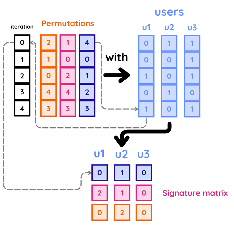
LSH starts with a so-called minhashing step, here a ‘signature matrix’ is being created through first performing random permutations of lists with values 0 to the number of movies. and then for each user, find the minimum value in each of the permutations that has been performed. Meaning that every user has as many values in their signature matrix row, as the number of permutations that have been performed, and each of these values are a found minimum with the minimum value associated with one of the movies that the user must have seen.
Inuition: Given that the minimum value is based on one of the movies the corresponding user has seen, and the value is essentially random, you can imagine that users that have seen many movies will end-up with lower values in their row in the signature matrix. Since for those users, there are more “random rolls”. It’s identical to rolling random dice rolls and choosing the minimum, the more dice rolls someone can do, the higher the probability that their final value is lower than someone with less dice rolls.
The main goal for this part of the algorithm is to mimic the data-matrix, by creating a smaller signature matrix, where pairs of users that have a high jaccard similarity with each other, will also have a higher likelihood of having an identical row in the signature matrix(!)
And this increased probability is abused in the next step, by using locallity sensitive hashing, the heart and soul of the algorithm. Now that there is a signature matrix with rows that might be identical, the next step is to “match” these rows, otherwise checking everything would still yield a full enumeration of $1.1 * 10^{10}$ pairs. Instead, LSH is used, which works by creating “buckets” of users, and these buckets are filled based on a specific label of the user, and this label is created by hashing the row of the user in the signature matrix. Hence, users with the same row in the signature matrix should get the same hash (with a small additional chance that a hash-collision occurs, but that probability is rather small). For these buckets, pairs have to be created in order to actually compare each of the pairs in the buckets, since possibly all of them could have a Jaccard similarity of at least 0.5 with each other, these are the candidate pairs.
Now to the final part of the algorithm, checking all of the candidate pairs. For each of the unique pairs that can be found in the buckets, check whether their true Jaccard Similarity is actually above 0.5. If it is, great! You can add that pair to the list, if not, too bad! It was a false positive.
The entire algorithm could then, in theory be repeated as long as time permits, and depending on the values for the number of total rows and the number of bands, the ratio of true positives to (false positives and false negatives) $\frac{TP}{FP + FN}$ changes, this is the ratio one is attempting to optimize through optimizing the number of bands and rows in the signature matrix.
Key Insight #1: Different bands are independent of each other
One must notice that given the algorithm, there must exist a single optimum that optimizes for $\frac{TP}{FP + FN}$, meaning there exists a single value for the number of rows in a band that must give the optimum. This then in turn means that the total number of rows must be precisely divisble by the number of bands, otherwise noise occurs by having a band that performs worse than the optimum.
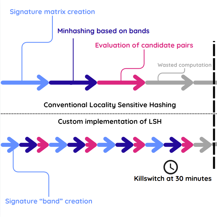
Then, since a single optimum exists for the number of rows and bands, one must then see that, since different bands do not interact with each other, they can be computed completely separately, in fact, the next band does not even need to be calculated before finishing the former. Therefore the “optimal signature matrix” can be considered a generator list that just outputs a few rows every once in a while.
This saves a LOT on the memory footprint of the algorithm, at the cost of little performance (more writes to disc) and ensures that even if the program running the algorithm would crash mid-computation somewhere in band 100, then the results of 99 bands would still be yielded.
This is opposite to the original idea, where a signature matrix would need to be perfected, with a certain maximum size, that is below 8 GB, and also able to finish within 30 minutes.
This new proposal abolishes this by generating the optimized rows, and giving the garbage collector (GC) the chance to remove unnecessary data still in memory. Ensuring that the memory footprint will always be well below the 8GB, and a new band can “greedily” be generated until time is up, instead of waiting patiently for the program to finish all the different bands at once.
Key Insight #2: Minhashing can be performed a lot faster given the specifics of the data
The original algorithm for minhashing attempts to find the minimum in a list of values (based on the movies), for each user, for each permutation. For 100 users and 1,000 movies, this means looping over 100,000 values for each permutation regardless of how many movies a user has watched.
This is pretty wasteful since only a single value needs to be returned for each user per permutation, and as long as the same value would have been returned by the “algorithm” it can be replaced by something better. Here we abuse some feature of the data, and also probability theory, in particular with the following: given a list of $x$ positives and $y$ negatives, what is the probability of finding a single positive value after $i$ iterations?
\[1 - (\frac{y-(i-1)-x}{y-(i-1)})^i\]For 17770 movies, and a user with 300 movies watched (the minimum), there is a 50% chance of finding a valid value after 41 iterations, after 175 this value exceeds 95% and after 397 it exceeds 99%. Meaning on average, only $\frac{42}{17770}=0.002$ of the total movies in the list have to be checked in order to get a value for a user in the signature matrix. And even in the 1% of cases where it exceeds 397, it will still be a lot lower than 17770, and the worst case is 17470 which is still lower than the original algorithm.
Intuition: The easiest way to visualise this in the brain is that given 3 positives and 7 negatives, in the permutation, all the values will be scattered around. Through the 3 positives, 4 segments can be created: before the first positive, in between the first and the second positive, in between the second and the third positive, and after the third positive. On average, the distance between the these positive points will be identical, meaning that the four segments are all equally large, meaning that roughly only 10/3 have to be performed to get a 63.2% chance of finding a positive ($1 - \frac{1}{e}$ euler(!)).
Now the only thing left is to implement an algorithm that applies this in some way, luckily there exists a mapping from the minimum value of a non-sorted list, to one that is sorted, they will look as the following:
original_permutation = [3, 1, 2]
permutation_sorted = [2, 3, 1]
If one were to use the permutation_sorted they would know that, when they find a positive value (i.e. the user has watched this movie in the permutation) then the found value must be the minimum.
Now, you should also notice that the values that are present in both lists are identical, meaning that the second is also just a permutation of the data, meaning that we can just interpret the first permutation as though it is the second! Now, we getting those nice properties of probability.
Original
--------------
BenchmarkTools.Trial: 1 sample with 1 evaluation per sample.
 Single result which took 13.145 s (0.00% GC) to evaluate,
 with a memory estimate of 5.56 MiB, over 23 allocations.


New Proposed Algorithm
--------------
BenchmarkTools.Trial: 26 samples with 1 evaluation per sample.
 Range (min … max):  152.432 ms … 231.201 ms  ┊ GC (min … max): 0.00% … 0.00%
 Time  (median):     203.225 ms               ┊ GC (median):    0.00%
 Time  (mean ± σ):   200.450 ms ±  19.031 ms  ┊ GC (mean ± σ):  0.00% ± 0.00%

  ▁▁                 ▁   █    ▁ ▁   ▁█ ▁▁█▁▁ ▁▁█ ▁▁▁    ▁  ▁  ▁
  ██▁▁▁▁▁▁▁▁▁▁▁▁▁▁▁▁▁█▁▁▁█▁▁▁▁█▁█▁▁▁██▁█████▁███▁███▁▁▁▁█▁▁█▁▁█ ▁
  152 ms           Histogram: frequency by time          231 ms <

 Memory estimate: 5.56 MiB, allocs estimate: 23
A speedup of at least 60 times(!).
Micro Optimization #1: using Booleans
Using Booleans instead of sparse matrices, or sets with integer values. Even though the data can be quite sparse, even for vectors, looping through boolean-type vectors is an order of magnitude faster than performing the computation on integers.
Of course, at some point the sparse-ness of the matrix wins over the speed upgrade from using booleans.
typeof(a) --> Vector{Int64}
typeof(b) --> Vector{Bool}

@benchmark sum(a)
BenchmarkTools.Trial: 10000 samples with 1 evaluation per sample.
 Range (min … max):  12.962 μs … 52.542 μs  ┊ GC (min … max): 0.00% … 0.00%
 Time  (median):     13.094 μs              ┊ GC (median):    0.00%
 Time  (mean ± σ):   13.427 μs ±  2.473 μs  ┊ GC (mean ± σ):  0.00% ± 0.00%

  █▃                                                          ▁
  ███▇▄▄▁▁▁▃▆██▄▅▃▅▃▃▃▁▃▁▁▃▁▁▁▁▁▁▁▁▁▁▁▁▁▁▁▁▁▁▁▁▁▁▁▁▁▁▁▁▅▆▆▅▅▄ █
  13 μs        Histogram: log(frequency) by time      26.9 μs <

 Memory estimate: 0 bytes, allocs estimate: 0.

-----------------------------------------------------------------------------

@benchmark sum(b)
BenchmarkTools.Trial: 10000 samples with 10 evaluations per sample.
 Range (min … max):  1.622 μs …   5.618 μs  ┊ GC (min … max): 0.00% … 0.00%
 Time  (median):     1.624 μs               ┊ GC (median):    0.00%
 Time  (mean ± σ):   1.667 μs ± 260.322 ns  ┊ GC (mean ± σ):  0.00% ± 0.00%

  █▂▁▁      ▁                                                 ▁
  ██████▇▇▇██▇▆▅▅▄▄▁▄▃▁▁▁▃▁▁▄▁▁▁▁▃▁▄▄▄▃▄▄▄▄▃▄▄▁▁▃▃▁▃▁▄▆▆▅▄▄▃▅ █
  1.62 μs      Histogram: log(frequency) by time      3.05 μs <

 Memory estimate: 0 bytes, allocs estimate: 0.

sum(a), sum(b), length(a), length(b)
50094, 50094, 100000, 100000
Micro Optimization #2: Using a fast programming language for all computing steps
Performance for Python using numpy is quite high when compared to standard Python, however not all steps can be done with numpy, and if a solution is suitable to be written entirely in numpy it will not be as readable as just using a language that has similar performance to numpy and works with the basic syntax. The original code in Python was written moreorless with numpy doing the heavylifting with Python gluing the code together. For comparison, the Julia method is also written to see how performance would change with an identical solution.
Final Idea: Using multiple threads
The final stage of serious optimization is of course using the multiple cores on one’s computer. For the Julia implementation this was achieved, and ran with 6 cores instead of 1. Although the only parallel part of the algorithm that was implemented was for checking whether the candidate pairs were true or false positives, since this process takes the longest time in the analysis. In theory, the entire program could be ran in parallel and then leaving a few seconds to combine the results of the different cores, since the problem is perfectly parallel.
Extra: Running the code on exceptionally weak hardware
The single-core Julia implementation of the LSH algorithm has also ran on exceptionally weak hardware with the AMD A9 (2 threads) with 4GB of RAM inside a 2017-era budget laptop. To see to which extend the Julia implementation is functionable on weaker hardware.
Background on Hardware
Hardware configurations
| CPU (threads, cores) | RAM (GB) | Single Core Performance (CPU benchmark) |
|---|---|---|
| Intel i5-8400 (6, 6) | 40 | 2367 |
| Intel i5-10210U (8, 4) | 36 | 2115 |
| AMD A9-9425 (2, 2) | 4 | 1323 |
Results
The most important figure is of course the progression of the different configurations over time. With the color indicating the programming language used, with the CPU name, the C6 indicates that 6 cores were used during computation.
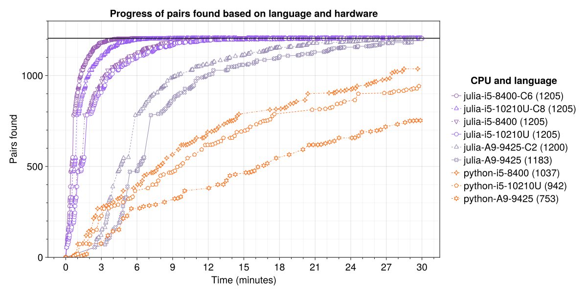
In this figure we can see that the Python implementation is able to find approxmimately 1000 pairs, and each of the julia implementations around 1200. More specifically, the AMD A9-9425 version is able to find 1200, while all other Julia configurations find 1205. Coincidentally, the ground truth of pairs with a Jaccard Similarity of strictly more than 0.5 is precisely 1205. Meaning the Julia implementation is able to find all the pairs that can be found in the data with sufficiently capable hardware. More specifically regarding the plot, we can see a line for each of the configurations that is akin to a log-plot, this is inherent to the algorithm and the data: since early in the program it is easier to find new candidates, while later in the program, the likelihood of finding duplicates is rather high. Consider 2 users with an identical movie list, these will always end up in the same bucket and form a candidate pair in each iteration. In each iteration of the program, it samples based on the Jaccard Similarity, those with a higher Jaccard Similarity have a higher probability of ending up in the candidate pairs, with pairs with lower Jaccard Similarity having a rather low chance of ending up in the candidate list. This means that it becomes increasingly more difficult to find new users, as virtually all remaining candidates are close to that 0.5 mark.
Now regarding the programs, in theory, the Julia implementation could have just “gotten lucky” with a specific seed. We can check this by looking at how many false positives the program found. If the Python program has a higher false positive rate than the Julia version, then the Julia version must have gotten lucky.
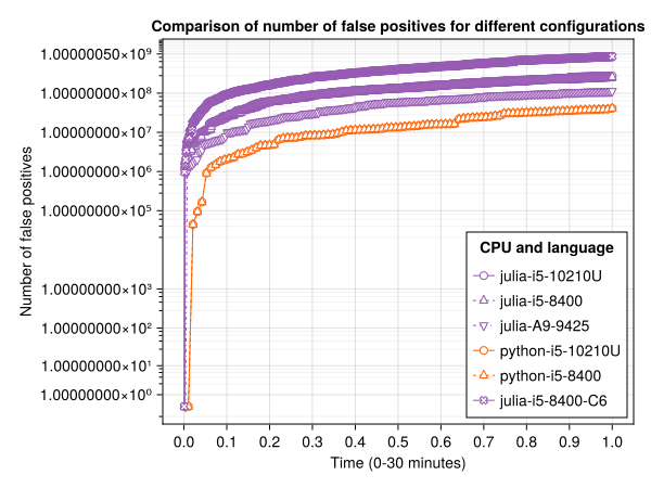
Gladly we do not observe that behavior at all, in fact, the Julia version finds strictly more candidates (both true and false positives) over time.
In the end, it is also technically possible for the number of duplicates to be higher in relation to new candidates, when plotting these values we get the following figure:
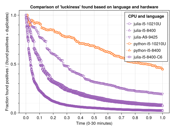
Here again, we see that the Julia version strictly outperforms the Python version, by consistently finding more duplicates in a short time, indicating that the Julia version indeed finds, and more importantly evaluates, many different candidates in a shorter time.
Even the AMD A9-9425 version with limited RAM and computing power using Julia is able to outperform a desktop CPU and more modern laptop CPU which use Python + numpy.
The 6-core multithreaded code is able to outperform the original single-threaded Python code in roughly 90 seconds. With each iteration being less than a second instead of almost 20s on average. This difference in performance is more pronounced in the next figure which shows the number of total iterations.
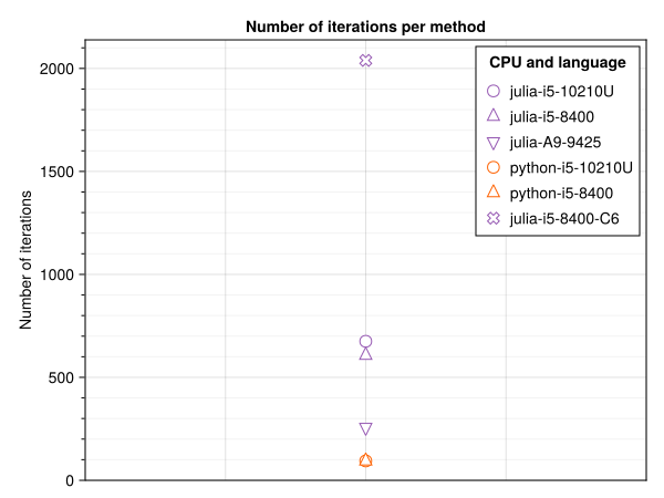
Although one must remain a little sceptical, since a seed could influence this value to a certain extend, and seeds between Julia and Python are not identical. Nevertheless the difference is substantial to such an extend that a seed would not change the overwhelming improvement of the Julia implementation.
Conclusion
Firstly, we can observe from the different results and optimizations that various algorithms can be changed or improved through some (over-)engineering, which can improve performance in specific workloads. Secondly, it is possible to observe that using a language that does not rely on an external library for performance, but has performance in the language ethos could improve performance through parts that are not very fast if using a 2-part system (i.e. the glue). Finally, through the improved performance, we can also observe that slower hardware with faster programs can outperform modern hardware running slower ones, (even when the algorithm’s solution is identical!), which gives a little nudge towards the idea, that perhaps, if we made our programs a little more performant, we wouldn’t need new computers as often as advertisements would suggest…