Creating an otter assembly pipeline
Creating an otter assembly pipeline using snakemake, commandline tools and Julia!

Background
Genome assembly has been around for quite some time. Starting from assembling simple organisms such as the Escherichia coli and the Saccharomyces cerevisiae. Only after the Human Genome Project (1990-2003), genome assembly really kicked off.
There are two broad ways of performing genome assembly. The first of which is the de novo assembly, which entails that all the reads that are created in a certain run are used in the process of assembly. One of the big problems with this technique is that it can be very computer intensive, since the overlap of reads is a very computer intensive task, let alone for over 3 million sequences in cases of small genome projects. Since one of the goals of this project was to make a genome assembler that could be run on someone’s laptop, the other technique is used: reference guided assembly. With the reference guided assembly technique, the reads that are found in a specific run are mapped to a reference genome, increasing performanc of the algorithm, and per extension making it possible to create genomes using a laptop.
| genome assembly method | pros | cons |
|---|---|---|
| de novo | unique links, truer information | computer intensive, slow |
| reference guided | highly performant, is able to perform variant calling more easily | needs a reference, wrong references leads to wrong results. |
After genome assembly, annotation can be performed, such as finding genes that are on the genome and researching how many chromosomes an organism has.
Why Sea otters?
Sea otters are adorable, I have watched many video’s of them over the years, and each one of them makes my heart melt. So for my spare time I wanted to find out what the otter genome is like. It should be stated however, that the pipeline still works on other organisms as well.
Unique aspects to the pipeline
A few characteristics that have been added to the pipeline are the following:
- All of the output files are stored in separate folders per category
- General overview of the fastq-reads file in a text-file
- Analysis of the quality per base in the reads file
- Analysis of the GC-distribution of the sequences
- General overview of the VCF-file in a text-file
- Analysis of the VCF-file with heatmaps per contig
Results
The following data were all results from the assembly of the Streptococcus ruminantium, since this organism was easy to perform assembly on, with quick feedback loops.
The input file of the reads was 1.5Gb, and the reference was 2.1Mb.
| input file | size |
|---|---|
| reads (DRR481114) | 1.5 GB |
| reference (NZ_AP018400.1) | 2.1 MB |
The head -6 can be found in the codeblock 1. Here it shows the read count, average length of reads, minimum length of reads (which surprisingly turned out to be zero), maximum length of reads, the average quality of reads and the average GC%. This particular script is the analyser.jl script, which took around 10s to run on this data, results of performance may vary due to incosistent read lengths.
Codeblock 1: The head -6 results of the analysis of the reads-file using analyser.jl.
It shows the read-count, average length of reads, minimum length of reads, maximum length of reads, average quality of the reads and the average GC%.
Read count:			 115352
Average length of reads:	 6263.98
Minimum length of reads:	 0
Maximum length of reads:	 263040
Average quality of reads:	 16.613954385095916
Average GC%:			 40.86%
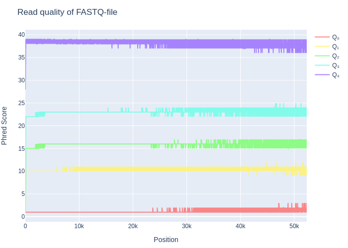
The quality was also plotted in the QC-plot which can be found in figure 1. This figure broadly shows all the different qualities that could be found on each of the different positions, with their minimum, maximum, Q1, median & Q3-values being shown.
Figure 1: The QC-plot. It shows the Minimum, maximum, Q1, Q3 and median values for each read position (in case the position has more than a thousand reads). Notice how the quality of the reads steeply increases in the first 10-100 bases. After 20k bases, the read length becomes a little more inconsistent and therefore all the values fluctuate on their qualities.
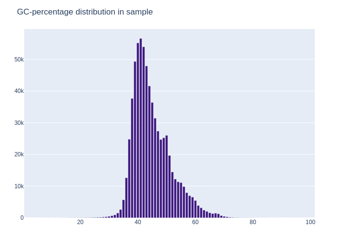
Besides the QC-plot there was also a GC-distribution plot, which labeled each of the sequences in buckets. The distribution of each of the percentages was then plotted. This plot can show contamination in the data, when there is a double peak found in the dataset. In the example case with the data from the lutra lutra, this was not the case, the plot showed a curve similar to that of the bell curve, meaning that the data was not likely to be contaminated.
Figure 2: The GC-distribution plot of the example Lutra lutra dataset. Here it shows a curve similar to that of a bell curve, signifying there was no significant contamination of foreign DNA in the dataset that was provided.
The general view of the VCF-file can also be found in the VCF-analysis text file. Which shows the SNP and INDEL mutations in the VCF-file.
An example output can be found in codeblock 2. In this example we can see that, on average, there are 3 deletions per insertion in our sequences when compared to the reference.
Codeblock 2: The example VCF-file on the S ruminantium. It possible to view the insertions, deletions, the indel-rate and the different SNP-mutations.
Insert count: 18
Deletion count: 54
INDEL-score; Insertion : deletion,  1 : 3.0
Mutations:
 				FROM
	--------------------------------------------------
		|	A	C	G	T
		|	----------------------------------
		| A	0	16	40	28
	TO	| C	6	0	5	71
		| G	77	5	0	10
		| T	9	55	16	0
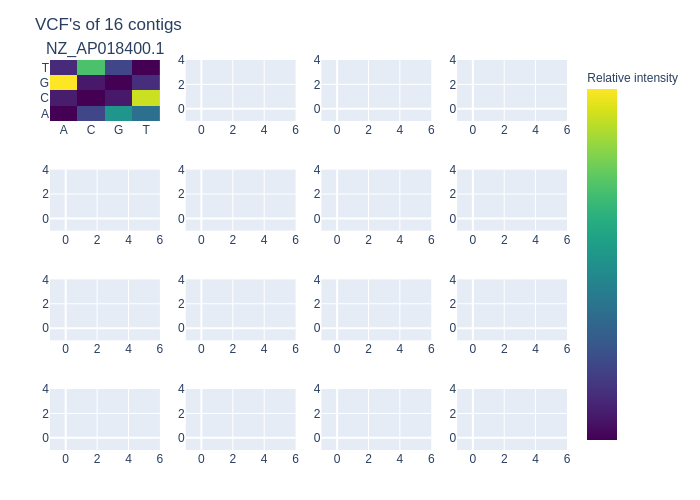
There was also an analysis of the VCF-file in a plot. This can be found in figure 3. In this heatmap plot it shows the relative SNP mutation on each of the contigs of the reference. Only 16 contigs could be loaded onto a single image. This means that there will be ceil(n / 16) plots with a minimum of 1. Showing the SNP mutations per contig.
Figure 3: The heatmap VCF-plot which shows all the relative counts of the SNP mutations in each of the contigs. Since the S ruminantium had only a single contig with its entire genome. There was only one heatmap filled in the 4*4 grid of heatmaps.
Performance
As earlier stated, the following data was used in testing the pipeline:
| input file | size |
|---|---|
| reads (DRR481114) | 1.5 Gb |
| reference (NZ_AP018400.1) | 2.1 Mb |
Using the following commando on the Swift 3 SF314-41:
time snakemake --cores 8 --snakefile Snakefile --use-conda all -F
forcing the snakemake pipeline to be run from start to finish, using the conda environment and having 8 cores to its disposal while also timing the duration of the run.
These were the results for a single particular run:
| measurement-type | time to completion (mm ss) |
|---|---|
| real | 71m 54s |
| user | 51m 29s |
| sys | 23m 07s |
It should be stated that most of this time is downloading the reads and the reference, mapping these references and then creating the vcf-file from the bam-file.
The measurements of each of the julia scripts can be found in table 2. From this, we can conclude that the julia scripts that were added to the pipeline did not alter the overall performance of the pipeline greatly, while also adding clearer insight into the data of that the pipeline provided. For the Lutra lutra part of the pipeline, it took around 24 hours to create the VCF-file. The VCF-file is therefore a lot (32x) bigger than the Streptococcus ruminantium version. This in turn also increased the time that the scripts needed to run for.
For the Lutra lutra dataset the following data was used:
| input file | size |
|---|---|
| reads (ERR3313341) | 18.7 GB |
| reference (taxid: 9657) | 2.5 GB |
table 2: Time measurements of each of the julia scripts that were added to the LOTRAP pipeline. Notice how the VCF-analysis script is noticably faster than a second.
| script | time (s) (Streptococcus ruminantium; reads: 1.5 GB; vcf: 91.2 kB) | time (s) (Lutra Lutra; reads: 18.7 GB; vcf: 2.9 MB) |
|---|---|---|
| analyser.jl | 9.286s | 113.856s |
| fastq_analyser_plot.jl | 132.301s | 563.646s |
| vcf_analysis.jl | 0.004s | 0.034s |
| vcf_plot.jl | 7.072s | 8.612s |
| sum | 148.664s | 686.148s |
By having created this pipeline, it has become possible for an average bioinformatician with a laptop with at least enough RAM, to perform the initial assemblation step of bio-informatics and analysis of the data sequence files.
The original code for this project can be found here. When the pipeline is updated, the blog post will be updated as well with the new information.
Addendum
I have a suspicion after running the pipeline with the 18.7 GB reads from the lutra lutra that the time complexity of the pipeline does not scale in a linear fashion, specifically the creation of the VCF-file exploded in time from around 5 minutes to 24 hours. Which would mean that it is not recommended to use this pipeline on very grand scale projects where time is costly, and the weekends can not be used to finish pipelines. Consequently, running the pipeline on your daily driver should only be recommended on small datasets.